Part 3 of a 4-part series on Call Intelligence. Part 1 covered the end-to-end pipeline; Part 2 covered the structured summaries this model reads.
The scale is real: about 300 million calls a year. Every example, topic name, number and screen below is mock data created for illustration.
The question behind every contact center
To run a contact center well, you first have to answer one question: why are people calling?
Most contact centers rely on manual disposition codes that agents pick after each call. They’re slow to capture, inconsistent between agents, and usually too broad for real analysis. “Claims” tells you very little. “Asking why a claim was denied” tells you where to look.
The call topic model tags every call with topics from a fixed taxonomy of topic groups and topics, so they can be tracked, trended and acted on. That makes it the foundation for finding self-service opportunities and widespread pain points.
One subtlety up front: the model tags topics discussed in the call, whether the caller or the agent raised them. It isn’t limited to the caller’s original reason for calling.
Why not just ask an LLM for every call?
You might expect us to send every summary to an LLM and ask for its topics. At our scale, that’s the wrong tool for the daily job:
- Volume. About 820,000 calls a day. Each call is several components (one per intent, plus the concise summary), and good labeling needs two LLM calls per component. That’s millions of LLM requests a day just for topics.
- Consistency. Trends only mean something if the same call always gets the same topics. A fine-tuned classifier is deterministic; an LLM prompt can drift when the model version changes.
- Speed and cost. A classifier scores a batch of summaries in one forward pass on a GPU. Our daily run uses a Dataproc cluster with 4 NVIDIA L4 GPUs.
So the LLM is used once, as a teacher, and a smaller model, the student, does the daily work.
- Teacher: an LLM labels 10,000 structured summaries with topics, using carefully designed few-shot prompts.
- Student: a pre-trained XLNet transformer is fine-tuned on those labels as a multi-label classifier. XLNet is what runs every day.
The expensive, flexible model creates the labeled data. The small, specialized model applies it, and the same input always gets the same output.
Input: the structured summary, not the transcript
The model reads two sections of the structured summary from Part 2:
- the concise summary
- the call intents
Example input (mock):
Concise summary: The caller is trying to book an appointment with a dermatologist at a local clinic. Her first-choice doctor was fully booked, so she booked with a new doctor whose details may not be in the directory yet. The agent confirms the first doctor is in-network and explains that the new doctor’s information needs to be updated.
Intents: The caller wants to know if a dermatologist at the clinic is in-network. The caller wants to know if the clinic is part of the plan’s network.
Part 2’s prompt asks for granular, keyword-rich intents, so this input is already clean and focused. That’s a big reason the topic model works.
Stage 1: Labeling training data with an LLM
Split the summary into components
Each summary is split into components: one per intent, plus the concise summary. Each component is labeled on its own.
Two steps: group first, then topic
The taxonomy is large. Asking an LLM to choose from every topic at once invites confusion between similar topics. So each component goes through two LLM calls:
- Predict topic groups from a fixed list of high-level groups.
- Predict topics from only the candidate topics mapped to those groups. The group-to-topic map is curated by hand.
Narrowing the choices first means the second call picks from a short, relevant list instead of the full taxonomy. Each call has a cap on how many labels it can return:
| LLM call | Max predictions |
|---|---|
| Intent → group | 3 |
| Intent → topic | 1 |
| Concise summary → group | 3 |
| Concise summary → topic | 3 |
Two rules shape the output:
- One topic per intent. Each intent is a single question, so it gets exactly one topic.
- The summary adds, it doesn’t repeat. When labeling the concise summary, topics already found from the intents are left out of the candidates. The summary pass only picks up additional topics, such as something the agent raised.
Here’s the labeling flow for one call (simplified). The response schema limits answers to the candidate list, so the model can’t invent a topic:
import json
import backoff
from google.api_core.exceptions import ResourceExhausted, ServiceUnavailable

@backoff.on_exception(backoff.expo, (ResourceExhausted, ServiceUnavailable), max_tries=5)
def ask(prompt: str, choices: list[str], max_items: int) -> list[str]:
    """One LLM call that must answer with items from `choices` (or "None")."""
    resp = model.generate_content(
        prompt,
        generation_config={
            "temperature": 0.1,
            "top_p": 0.95,
            "response_mime_type": "application/json",
            "response_schema": {
                "type": "ARRAY",
                "items": {"type": "STRING", "enum": choices + ["None"]},
            },
        },
    )
    picked = [c for c in json.loads(resp.text) if c != "None"]
    return picked[:max_items]


def label_component(text: str, kind: str, exclude: set[str] = frozenset()) -> list[str]:
    """kind is "intent" or "summary"."""
    groups = ask(group_prompt(text), GROUPS, max_items=3)
    candidates = [t for g in groups for t in GROUP_TO_TOPICS[g] if t not in exclude]
    if not candidates:
        return []
    examples = pick_examples(text, EXAMPLE_POOL)
    return ask(topic_prompt(text, candidates, examples), candidates,
               max_items=1 if kind == "intent" else 3)


def label_call(summary: dict) -> list[str]:
    topics = []
    for intent in summary["call_intents"]:
        topics += label_component(intent["intent"], "intent")
    # The summary pass only adds topics the intents didn't already cover.
    topics += label_component(summary["concise_summary"], "summary", exclude=set(topics))
    return sorted(set(topics))
Few-shot examples chosen per input
The prompt includes hand-curated examples. Rather than using the same ones every time, the most relevant are picked for each input using n-gram overlap. Each prompt gets:
- at least 3 examples covering at least 2 different topics, and
- at least 1 example with no label, which teaches the model that “None” is a valid answer for noisy or off-taxonomy text.
import re

def ngrams(text: str, sizes=(1, 2)) -> set[str]:
    words = re.findall(r"[a-z0-9']+", text.lower())
    return {" ".join(words[i:i + n]) for n in sizes for i in range(len(words) - n + 1)}

def pick_examples(text: str, pool: list, k: int = 3) -> list:
    """Most similar labeled examples (>= k, covering >= 2 topics) plus one "None" example."""
    target = ngrams(text)
    ranked = sorted(pool, key=lambda ex: len(target & ngrams(ex.text)), reverse=True)

    chosen, topics = [], set()
    for ex in ranked:
        if ex.topic is None:
            continue
        if len(chosen) < k or (len(topics) < 2 and ex.topic not in topics):
            chosen.append(ex)
            topics.add(ex.topic)
        if len(chosen) >= k and len(topics) >= 2:
            break

    chosen.append(next(ex for ex in ranked if ex.topic is None))
    return chosen
The prompt (simplified)
You are a data labeler categorizing a caller's intent: any action the
caller takes or intends to take during a call with a health insurance
call center.

YOUR KNOWLEDGE IS STRICTLY LIMITED TO THE CALL INTENT AND THE EXAMPLES
PROVIDED. DO NOT MAKE ASSUMPTIONS BEYOND WHAT IS EXPLICITLY STATED.

From the candidate list, choose the topic that best describes the
caller's intent. If the intent does not match any candidate (too niche,
ambiguous, or undefined), respond "None".

Candidate topics and definitions:
{candidate_definitions}

Examples:
{best_few_shot_examples}

Intent: {intent}
Topic:
API settings
| Setting | Value |
|---|---|
| Model | Gemini-family LLM |
| Temperature | 0.1 |
| Top-p | 0.95 |
| Retries | Exponential backoff |
From labels to a training row
All topics predicted for a call are combined into one list. That becomes one row of training data: the input text, plus a 0/1 flag for every topic.
def training_row(summary: dict, topics: list[str]) -> dict:
    text = summary["concise_summary"] + "\n" + "\n".join(
        i["intent"] for i in summary["call_intents"])
    return {"text": text, "labels": [1.0 if t in topics else 0.0 for t in TOPICS]}
Checking the labels before training
A student can only be as good as its teacher. Before training, every label is checked: an LLM verifies whether the predicted topic is actually present in the summary. That gives a precision score for each topic, so weak topics are caught before any training happens.
Stage 2: Fine-tuning XLNet
Small and large topics
Topic volumes are very uneven. A handful of topics cover a large share of calls, while many others are rare. Train one model on all of them, and the frequent topics dominate while the rare ones get lost.
So topics are split by volume and trained as two separate models:
| Group | Definition | Training target |
|---|---|---|
| Small topics | Less than 1% of total calls | 0/1 vector over small topics only |
| Large topics | 1% of calls or more | 0/1 vector over large topics only |
In both cases the input is the same: the concise summary plus the call intents.
SMALL_TOPICS = [t for t in TOPICS if call_share[t] < 0.01]
LARGE_TOPICS = [t for t in TOPICS if call_share[t] >= 0.01]
Multi-label fine-tuning
Each call can have several topics, so the model is multi-label: it scores every topic on its own instead of picking one winner. With Hugging Face Transformers, that’s one setting, problem_type="multi_label_classification", which uses a sigmoid and binary cross-entropy per topic. A simplified version of the training job, run once for each topic set:
from datasets import Dataset
from transformers import (Trainer, TrainingArguments,
                          XLNetForSequenceClassification, XLNetTokenizer)

tokenizer = XLNetTokenizer.from_pretrained("xlnet-base-cased")

def to_dataset(rows: list[dict], topics: list[str]) -> Dataset:
    enc = tokenizer([r["text"] for r in rows], truncation=True,
                    max_length=512, padding="max_length")
    labels = [[r["labels"][TOPICS.index(t)] for t in topics] for r in rows]
    return Dataset.from_dict({**enc, "labels": labels})

def train(topics: list[str], train_rows, val_rows, out_dir: str) -> Trainer:
    model = XLNetForSequenceClassification.from_pretrained(
        "xlnet-base-cased",
        num_labels=len(topics),                       # one output per topic
        problem_type="multi_label_classification",    # sigmoid + BCE per topic
    )
    trainer = Trainer(
        model=model,
        args=TrainingArguments(out_dir, num_train_epochs=EPOCHS,
                               learning_rate=LR, per_device_train_batch_size=BATCH),
        train_dataset=to_dataset(train_rows, topics),
        eval_dataset=to_dataset(val_rows, topics),
    )
    trainer.train()
    return trainer

small_model = train(SMALL_TOPICS, train_rows, val_rows, "xlnet-small-topics")
large_model = train(LARGE_TOPICS, train_rows, val_rows, "xlnet-large-topics")
A cutoff for each topic
The model outputs a probability for every topic. A topic is assigned when its probability clears a cutoff. A single cutoff for every topic is rarely right, because rare and common topics behave differently, so each topic gets its own, chosen on held-out data to maximize F1:
import numpy as np
from sklearn.metrics import f1_score

def tune_thresholds(probs: np.ndarray, labels: np.ndarray) -> np.ndarray:
    """probs, labels: (n_calls, n_topics). Returns the best cutoff per topic."""
    grid = np.arange(0.10, 0.91, 0.05)
    return np.array([
        max(grid, key=lambda th: f1_score(labels[:, j], probs[:, j] >= th, zero_division=0))
        for j in range(labels.shape[1])
    ])
Running in production
Both models run as a daily batch on new structured summaries, about 820,000 calls a day. Because transcripts and summaries need to be complete first, topics land a few days after the call. The job writes one partition per day, so a rerun replaces that day instead of duplicating it, the same rule as every job in Part 1.
Inference on four L4 GPUs
Topic inference runs on a Dataproc cluster with 4 NVIDIA L4 GPUs. The day’s summaries are split into four shards, one per GPU. Each GPU loads both models (small and large topics) once and scores its shard in batches. Simplified:
import torch
import torch.multiprocessing as mp

N_GPUS = 4                                    # Dataproc cluster, 4 x NVIDIA L4

@torch.no_grad()
def predict(model, device, texts, topics, cutoffs) -> list[list[str]]:
    inputs = tokenizer(texts, truncation=True, padding=True,
                       max_length=512, return_tensors="pt").to(device)
    probs = torch.sigmoid(model(**inputs).logits)
    return [[topics[j] for j in (p >= cutoffs).nonzero().flatten().tolist()] for p in probs]

def score_shard(gpu: int, shard: list[dict], run_date: str) -> list[dict]:
    device = torch.device(f"cuda:{gpu}")
    large = load_model(LARGE_MODEL_PATH).to(device).eval()
    small = load_model(SMALL_MODEL_PATH).to(device).eval()
    large_cut, small_cut = LARGE_CUTOFFS.to(device), SMALL_CUTOFFS.to(device)

    rows = []
    for batch in chunks(shard, size=BATCH_SIZE):
        texts = [s["concise_summary"] + "\n" + "\n".join(s["intents"]) for s in batch]
        lg = predict(large, device, texts, LARGE_TOPICS, large_cut)
        sm = predict(small, device, texts, SMALL_TOPICS, small_cut)
        for s, a, b in zip(batch, lg, sm):
            rows.append({"call_id": s["call_id"], "call_date": run_date,
                         "call_topics": (a + b) or ["Unfiltered"], "run_time": now_utc()})
    return rows

def run_topics(run_date: str) -> None:
    summaries = [dict(r) for r in bq.query(SUMMARIES_SQL, job_config=params(run_date)).result()]
    shards = [summaries[g::N_GPUS] for g in range(N_GPUS)]       # one shard per GPU

    with mp.get_context("spawn").Pool(N_GPUS) as pool:
        parts = pool.starmap(score_shard, [(g, shards[g], run_date) for g in range(N_GPUS)])
    rows = [r for part in parts for r in part]

    bq.load_table_from_json(
        rows, f"contact_intel.call_topic${run_date.replace('-', '')}",
        job_config=bigquery.LoadJobConfig(write_disposition="WRITE_TRUNCATE"),
    ).result()
Output, one row per call:
| Field | Description |
|---|---|
call_id |
Unique identifier for the call |
call_date |
Date the call occurred |
call_topics |
List of topics predicted for the call |
run_time |
When the model ran for this call |
A separate topic hierarchy table maps each topic to its group. Keeping the hierarchy in its own table means topics can be regrouped or renamed for reporting without rerunning the model.
-- Count distinct calls per topic and group
SELECT
  h.topic_group,
  t AS topic,
  COUNT(DISTINCT o.call_id) AS calls
FROM contact_intel.call_topic o,
     UNNEST(o.call_topics) AS t
JOIN contact_intel.call_topic_hierarchy h
  ON h.topic = t
WHERE o.call_date BETWEEN @start AND @end
GROUP BY h.topic_group, topic
ORDER BY calls DESC;
Counting tip: because calls are multi-label, topic shares can add up to more than 100%. Count
DISTINCT call_idper topic, and say so on the dashboard.
“Unfiltered” calls
Some calls don’t map to any topic. They’re reported as Unfiltered rather than forced into the closest category. They come from two sources:
- Calls without content, such as calls disconnected within seconds.
- Calls about topics not in the taxonomy yet.
The first group is noise. The second is a signal: if Unfiltered volume grows, the taxonomy is missing something.
How we measure quality
The metrics, in plain language
- Precision: how often are we right? Put every call the model labeled “asking why a claim was denied” in a bucket. Precision is how pure that bucket is.
- Recall: how many did we find? Picture the whole river of calls. Recall is how many of the true “denied claim” calls the net actually caught.
- F1: the balance. It’s hard to maximize both at once. F1 measures how well you fill the bucket with only the right calls and catch most of them.
Step 1: Training data (machine check)
For each label the LLM produced, a second LLM check confirms whether the topic is really in the summary. Precision is calculated per topic, then averaged across topics without weighting, so rare topics count as much as common ones.
Step 2: Model (human review)
- Sample about 200 calls, chosen so every topic appears at least 10 times.
- For each predicted topic, a reviewer marks whether it’s actually present in the transcript (precision).
- The reviewer also notes topics in the transcript that the model missed (recall).
- Compute precision, recall and F1 per topic, then average across topics, again unweighted.
from sklearn.metrics import precision_recall_fscore_support

# y_true, y_pred: (n_reviewed_calls, n_topics) 0/1 arrays from the review sheet
p, r, f1, _ = precision_recall_fscore_support(y_true, y_pred, average="macro", zero_division=0)
average="macro" is the unweighted average: every topic counts once, however rare.
Two choices are worth copying:
- Stratified sampling (“each topic at least 10 times”) gives every topic enough examples to measure. A random sample would be mostly the top few topics.
- Checking against the transcript, not the summary, measures the whole chain end to end, including anything the summary missed.
Keeping it current
The model is re-evaluated every six months. Each cycle:
- improves accuracy for topics that are underperforming, and
- adds new topics based on user requests and emerging needs, often surfaced by the Unfiltered bucket.
Putting topics to work
Joined with operational metrics in the consolidated table (Part 1), topics show not just what members call about but what each topic costs:
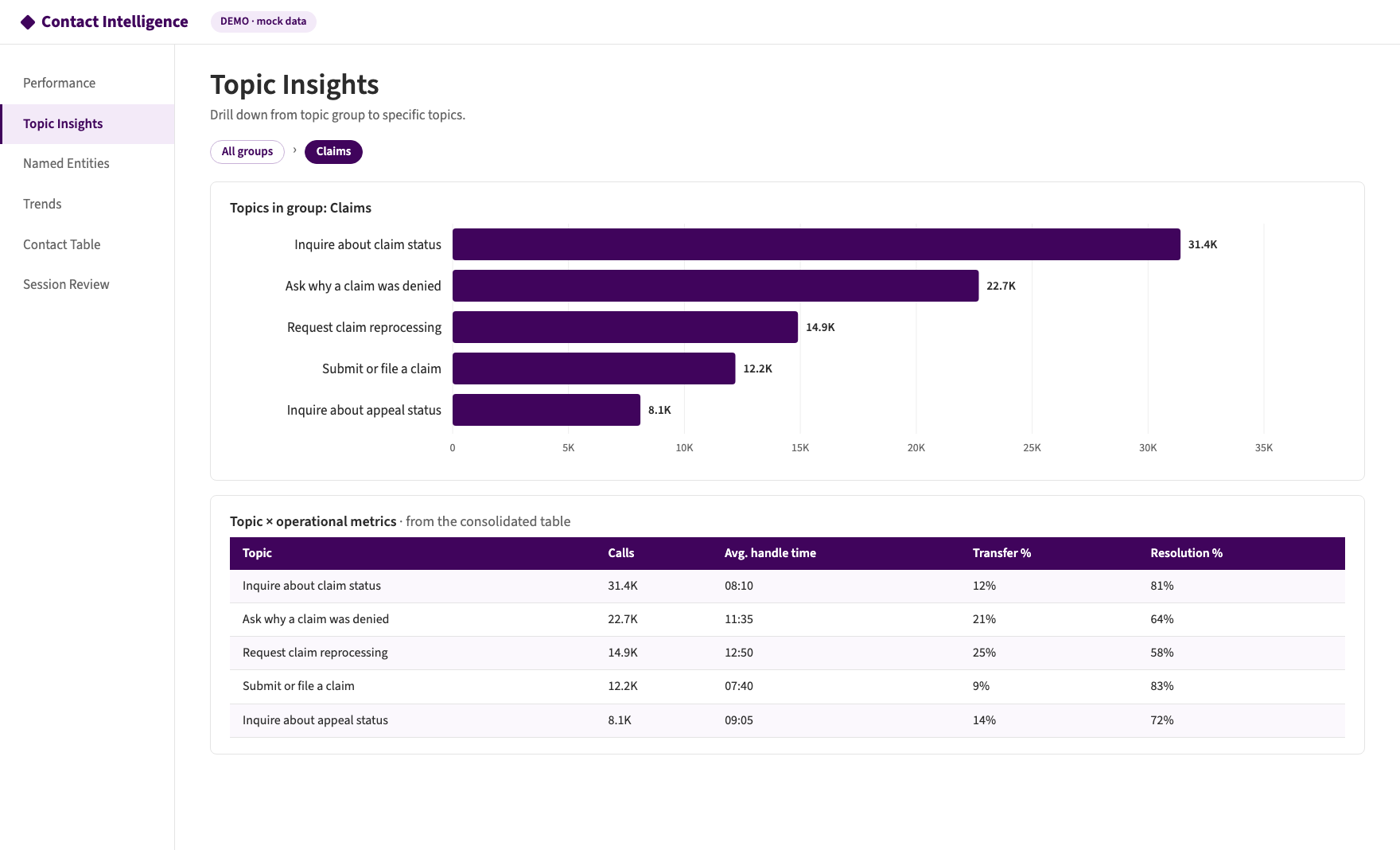 Figure 5: Drill-down from a topic group to specific topics, with operational metrics (mock data).
- High volume and simple → self-service candidates.
- High transfer rate or low resolution → broken handoffs or unclear processes.
- Rising trend → an emerging issue to investigate early.
- After a fix ships → watch that topic’s volume to measure impact.
Lessons learned
- Use the LLM as a teacher, not as the daily model. At hundreds of thousands of calls a day, let the LLM create labels once and train a smaller model to apply them.
- Narrow before you choose. Picking a topic group first, then a topic, beats choosing from the full taxonomy in one step.
- Constrain the answer. A response schema limited to the candidate list means the LLM can’t invent topics.
- Pick few-shot examples per input, and include a “no label” example so “None” stays a real option.
- Check the teacher’s labels. Errors in training data become errors in the model.
- Model rare and common topics separately. Otherwise rare topics disappear.
- Sample so every topic is measured, and average without weighting.
- Treat Unfiltered as feedback. It shows where the taxonomy needs to grow.